Have you ever wondered where you would be now if you had grown up in a different environment? Would you be healthy? More successful in your studies? Happier?

How do your living conditions affect your life?

This is the question we asked ourselves after reading how Mexico managed to improve children’s health and their mother’s happiness by replacing dirt floors with cement, in a program called Piso Firme ¹.

Indeed, achieving such results with only a bit more than 150$ of cement per household seemed rather encouraging, but this led us to wonder:

What is the impact of the housing environment on education, health & happiness?

What, where, who, when?

To try and answer that vast question we decided to focus on three main research axes.

Which life outcome (education, health or happiness) is most affected by which housing conditions?

What is the effect of precarious housing on health (both physical and mental) and school involvement for children?

Are there differences in the effects of precarity between different age groups? If so, for which outcomes?

To conduct this study, we opted for a subset of the data from the National Survey of America’s Family ² of 2002, to see the perspective from the other side of the frontier, in a similar timeframe as Piso Firme (the program started in 2000). We combined data from children aged 6 to 17 and their respective households.

This dataset recenses a large number of households throughout the USA, providing insight on their demographics and health indicators of the inhabitants.

Are you ready? Let’s dive in!

General influence of living conditions on education, health & mental health

First, let’s have a look at which housing conditions impact which life outcome the most.

How?

To find the relationship between housing conditions and education, health and mental health, we perform linear regressions. Living conditions are defined as a number of various indicators such as housing (own or rent, overcrowding), family situation (structure, relationship with parents, parents mental health), income, extrascolar activities and personal caracteristics (sex and age).

Education

Our indicator for education is measured on a school engagement scale, higher score meaning greater engagement in school (for example, a child that always does his homework willingly, is interested in learning and does well in school).

Let’s look at some of the features that seemed to influence involvment in school the most.

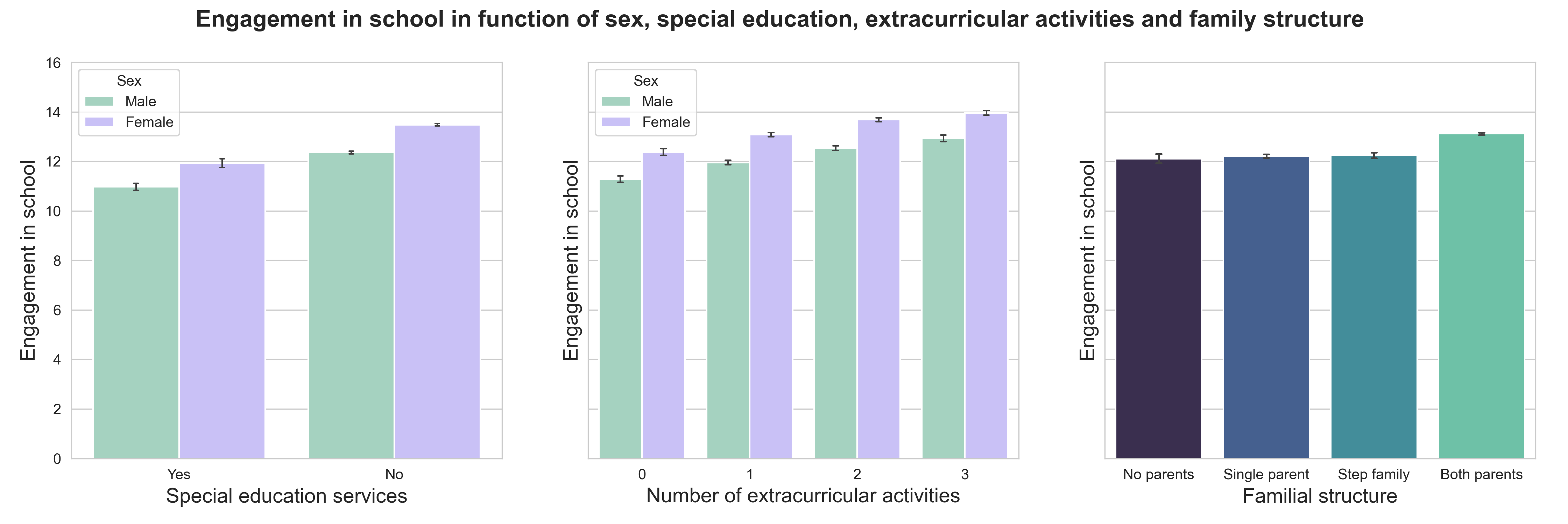
As we could expect, children receiving special education services (on the left) show less engagement in school than children who don’t.

The middle plot shows that children who take part in more activities outside of school, like sports, lessons or any kind of clubs, seem to be more involved (so go get that gym membership that you’ve been talking about for months!).

It is also interesting to note that girls are definitely more engaged in school than boys!

The effect of family structure also seems to play a role as we can see on the right. Even though the first three living familial arrangements do not show any particular relationship with education, it seems that children living with both parents are more involved in school work.

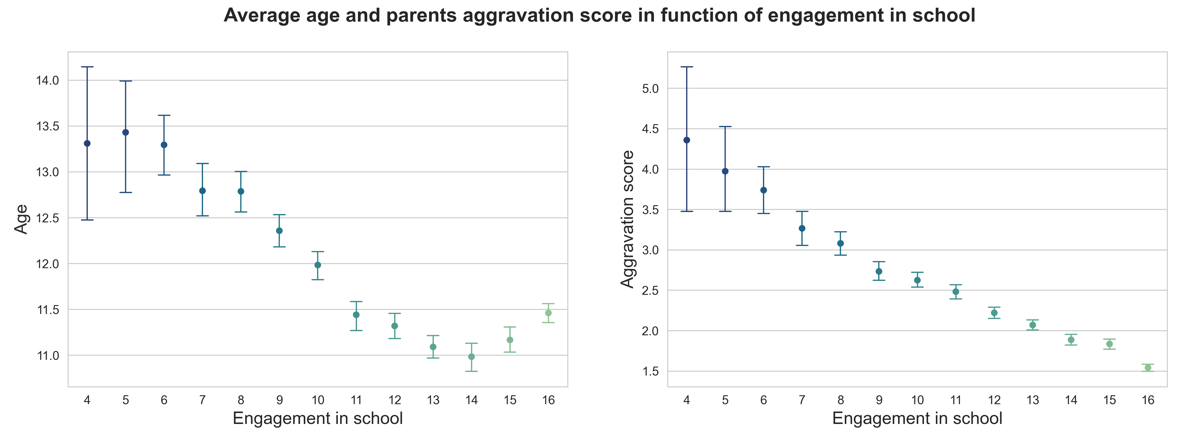
This plot on the left shows a compelling story. From a general point of view, it seems that highly engaged children are younger than less engaged ones. An explanation could be that as children grow older, their parents will likely supervise their school work less. However, we can see that the mean age of the most engaged children (15+ scores) is higher, meaning, perhaps, that some of the more involved students show high engagement for their entire education, regardless of age…

Lastly, let’s talk about the aggravation score. This is an indicator of the aggravation of the relationship with the parents, higher scores indicating worse relationship. Unsurprisingly, school engagement linearly increases with better parental relationship.

Physical health

The indicator for physical health that we used was a scale representing the current health status ranging from 1, excellent, to 5, poor. We will thus refer to it as the poor health indicator as higher values refer to worse physical condition.

Here are some of the features with the most influence on health:

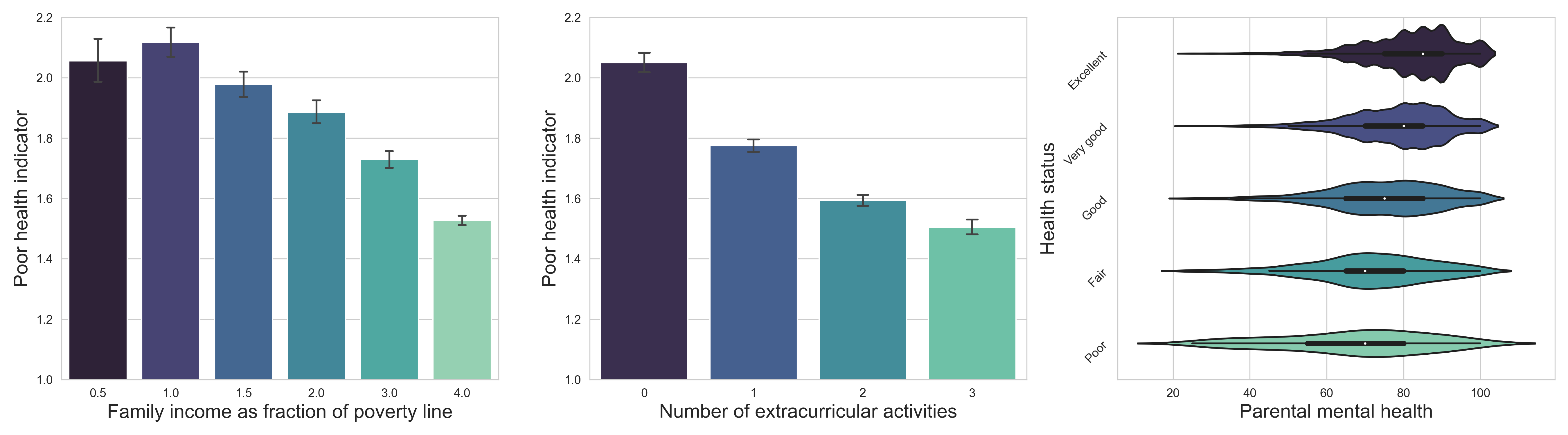
First, we can observe that higher family income is related to less health issues. However, it would be interesting to study this effect in more details, as it is certainly linked to other factors. For example, poorer family perhaps do not have the insurance coverage needed to resolve their children’s health problems if they have any.

In a second time, we can see in the middle that children that take part in many activities outside of school are in better physical condition. Again, we do not know if doing less activities (sports for instance) leads to poorer health or if it is the poor health that limits activities.

Finally, we show the distribution of parental mental health (higher scores indicating better mental health) in function of children’s health status. As children’s health deteriorate, so does the mental health of parents. That would make sense, as the health of children is definitely a big concern for the parents.

Mental health of children

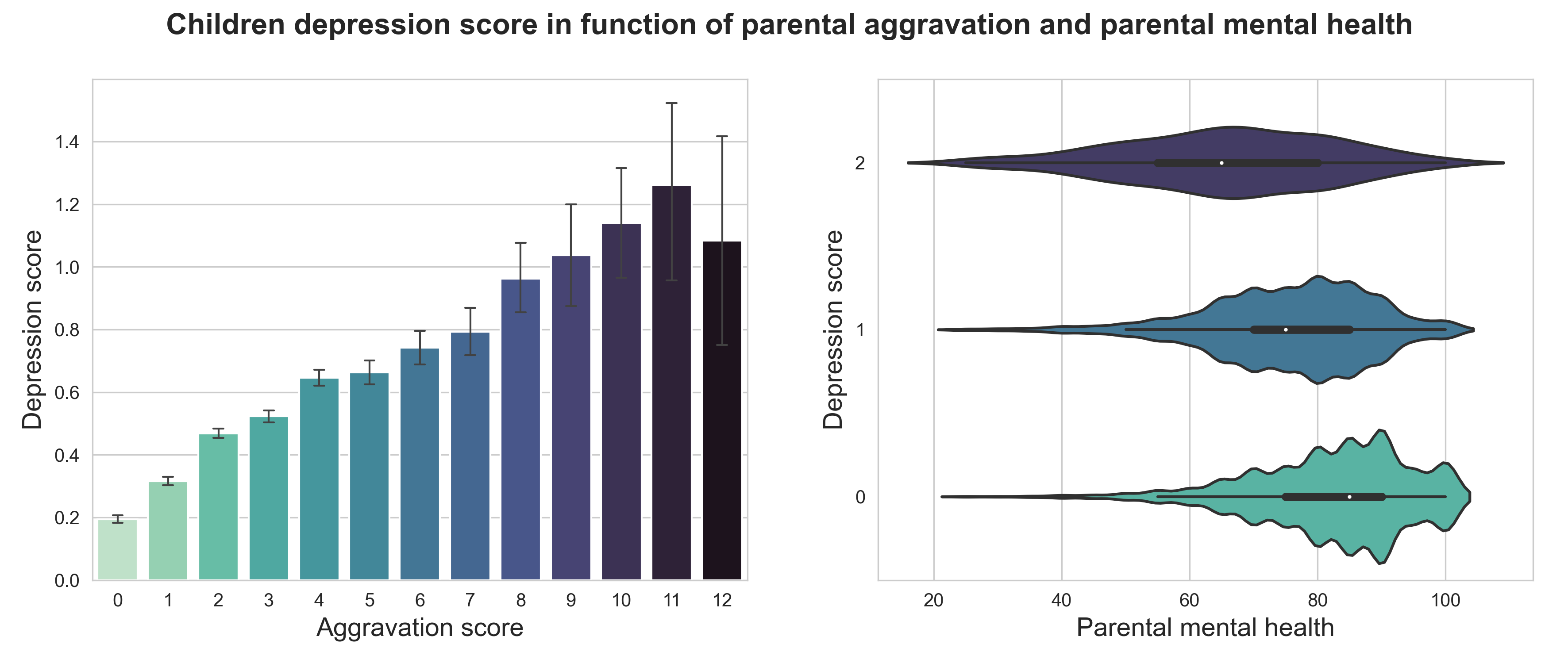
Now let’s see whether depressive feelings are linked to the environment in which the children evolve. We use a depression score that ranges from 0 to 2, lower scores indicating happier children.

Here are shown the conditions that impact chilren well-being the most:

Let’s take it step by step!

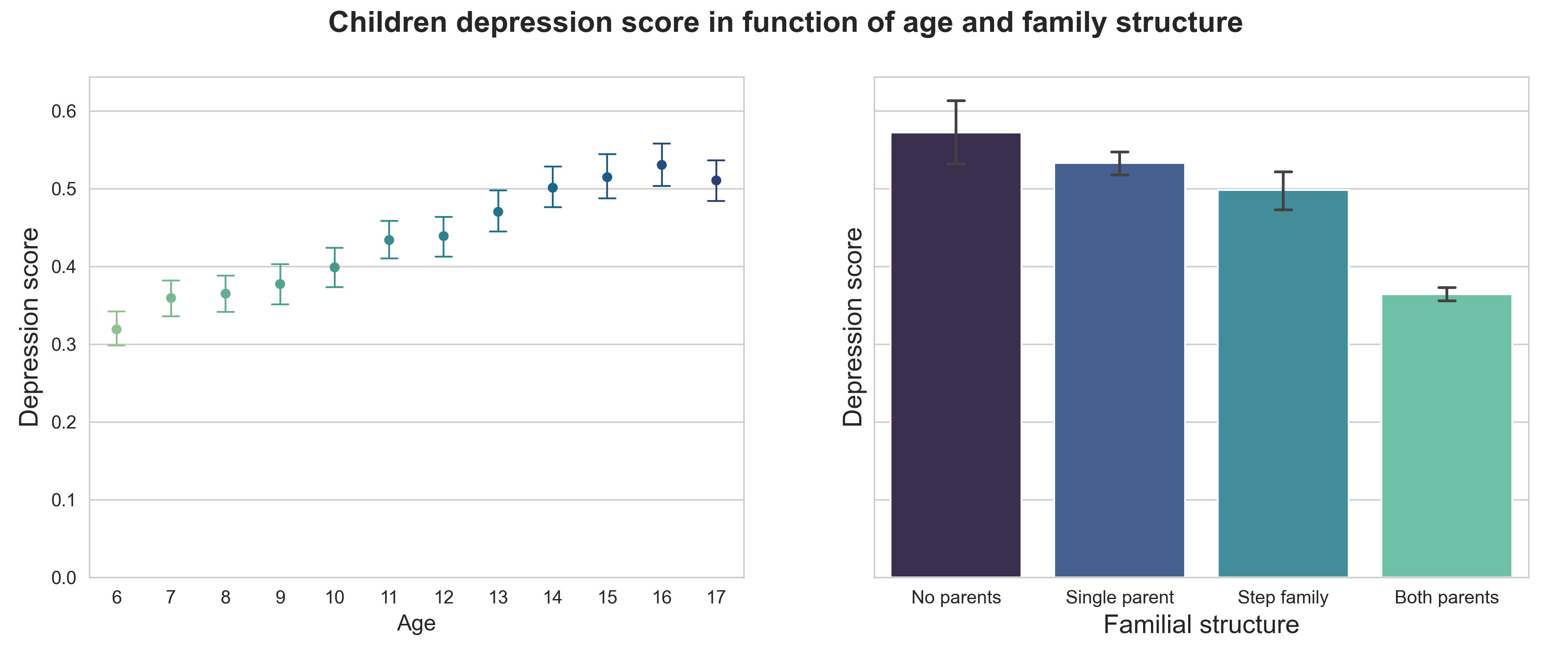
First, let’s look at the evolution with age. Sadly, it shows that the mental health of children steadily deteriorates with age. The trend seems to reach a plateau at around 16, which coincides with the end of adolescence. It can be quite a troubling period for many teenagers, which might explain this increasing occurence of depression between age 10 and 16. It would be interesting to see the results to see if depression rate decreases after that (hopefully it does!).

Now, looking at the link with family structure, we observe that as it improves, so does mental health, which seems quite logical.

The aggravation is clearly correlated with depression in children. However, it is difficult to establish the link of causality between them - does depression leads to deterioration in relationship with parents or does a bad relationship causes to develop depressive feelings for the child?

Lastly, the distribution of parental mental health scores in function of children’s well-being shows a positive correlation as well. It is difficult to say whether this is due to a common living condition (bad housing for instance) which influences the mental health of the entire household, or if the well-being of one person impacts the well-being of the other.

Mental health of parents

Out of curiosity, we decided to look briefly into the influence of living conditions on parents happiness. It turned out that income, relationship with children and having a disabled child seemed to play a role.

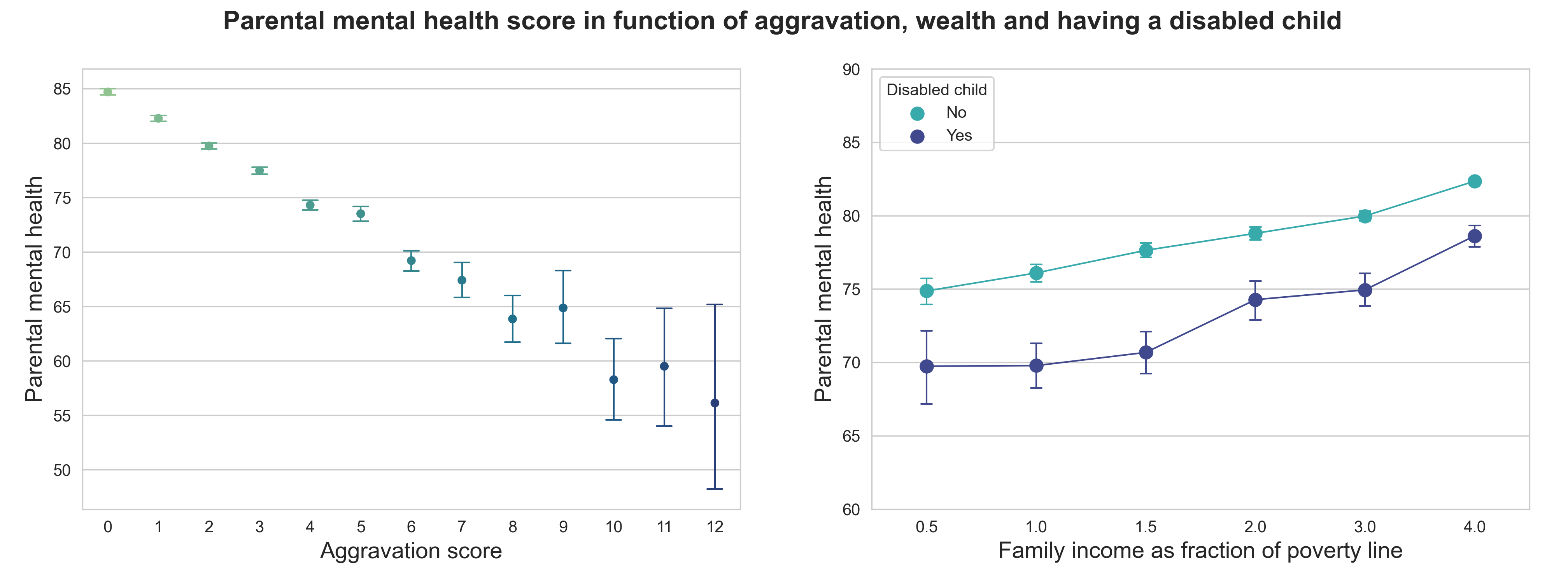
Without surprise, parents mental health deteriorates as the relationship with children worsen. But again, causality is hard to establish…

Now, let’s look at income and having a disabled child (physically or mentally) at home.Regardless of that last parameter, higher income correlates with happier parents. Does that mean that money can buy happiness? Let’s not jump to conclusions, there are many variables linked to income that were not taken into account here…

However, another interesting thing from this plot is that having a disabled child seems to negatively impact parents mental health (parents with a disabled child are about 10% less happy than parents with healthy children), which could be due to a lot more of responsibilities and time spent to care for this child. Being a parent is a full-time job!

Influence of precarious living conditions

Next, let’s dive deeper and compare life outcomes of people living or not in precarious conditions.

How?

To start with, we need to determine what ‘precarious conditions’ actually means for our study. To do so, we established a living index reflecting the quality of life, based on variables both economic (income, house ownership, health insurance) and social (family structure, relationship with parents, overcrowding). Then, looking at the distribution of this index we decided on a threshold splitting the initial population into two subpopulations, precarious or non-precarious.

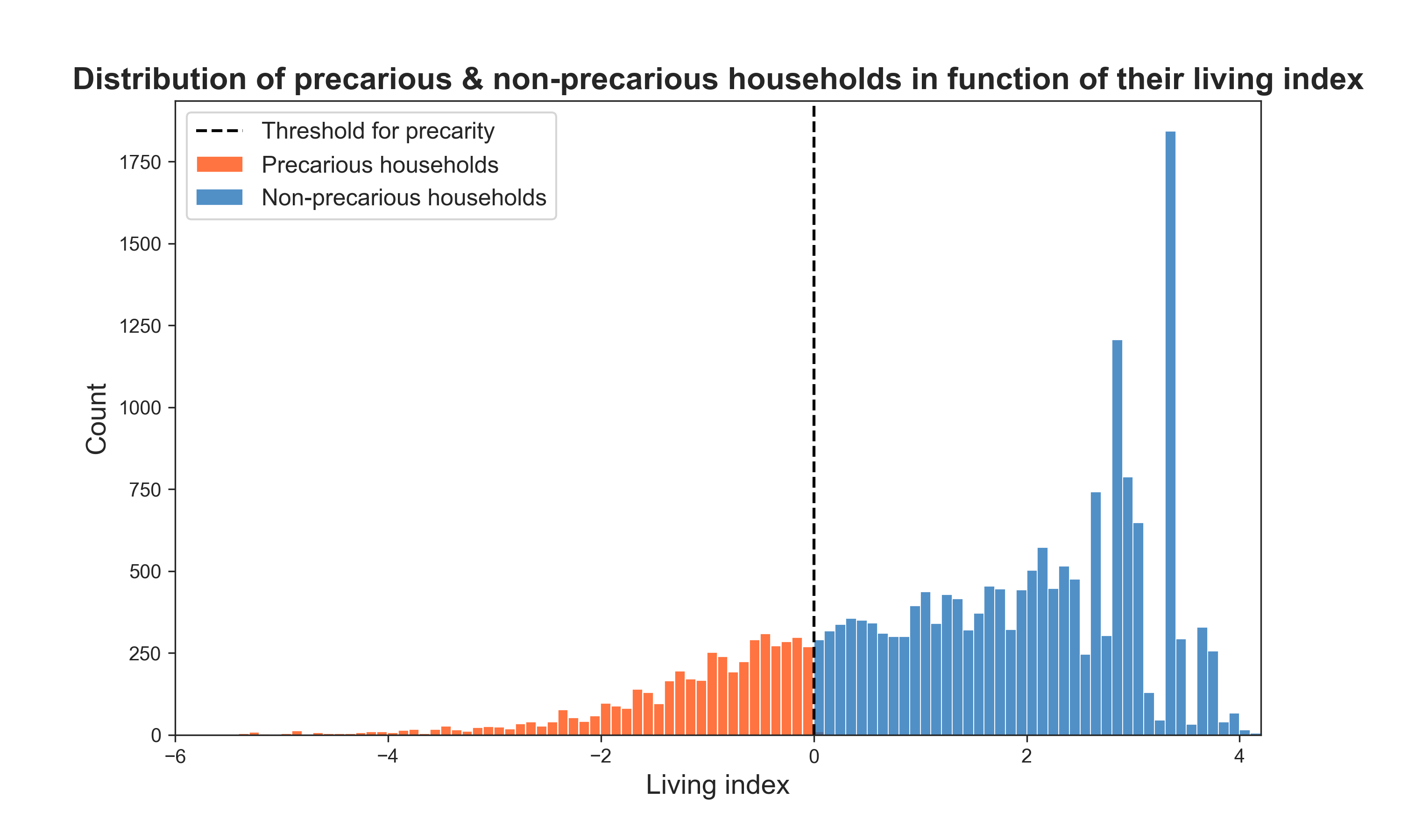
Around 25% of children were assigned to a precarious household.

Propensity score matching

Now, we could simply compare education scores between children from precarious and non-precarious households. However, this would not account for the effect of many other variables that also play a role, such as the ones we showed above.

The idea would be to compare children that are similar except for the fact that they live in a precarious household or not. Thus, we need to compute what is called a propensity score, which represents the probability of being assigned a treatment given a set of variables. Then, we can match children from different subpopulations that have a similar propensity score.

Let’s go through it together!

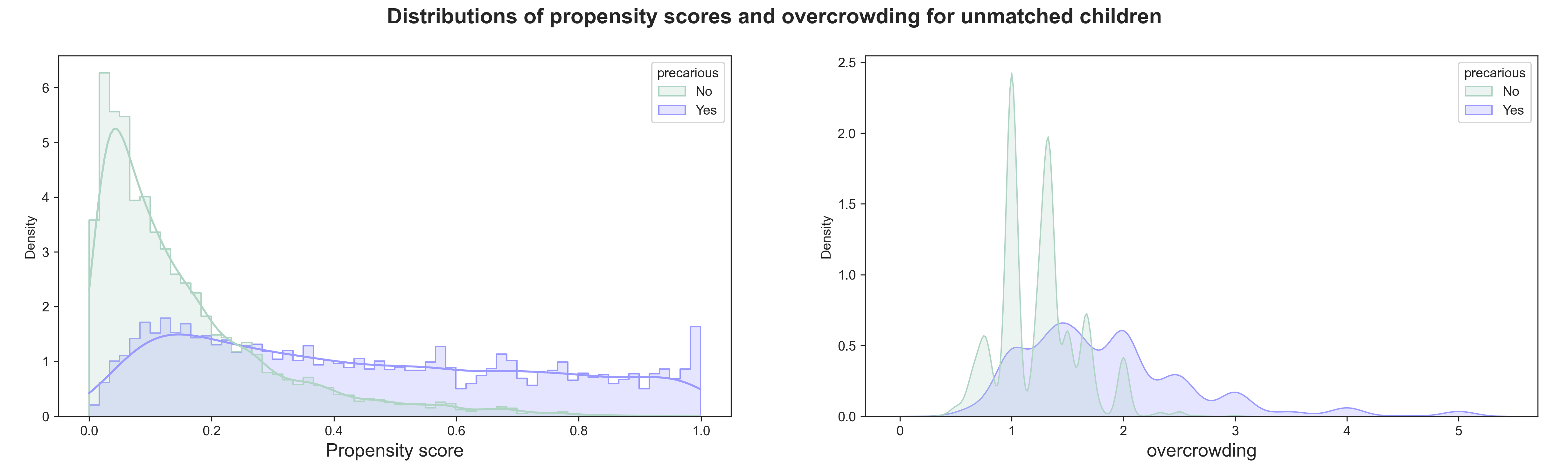
Let’s consider the two groups of children that we constituted earlier, one living in precarious conditions while the other does not. We can compute a propensity score based on a large number of other variables, personal (sex, age, region, activities), familial (parents highest educational degree), housing (overcrowding, number of people in the household, number of rooms) and health (disability).

Take a look at the distribution of the propensity scores among the two groups before matching: it is not evenly distributed. Let’s look at the distribution of one of the variables, overcrowding, in these two groups as well: again, not identical.

Now, we can perform matching, that is we find pairs of children coming from different groups but with very close propensity scores.This means that these children are very similar regarding all the above-mentioned variables but differ by the treatment (living in precarious conditions). Let’s have a look again at the distribution of propensity scores and the overcrowding variable over the two groups.

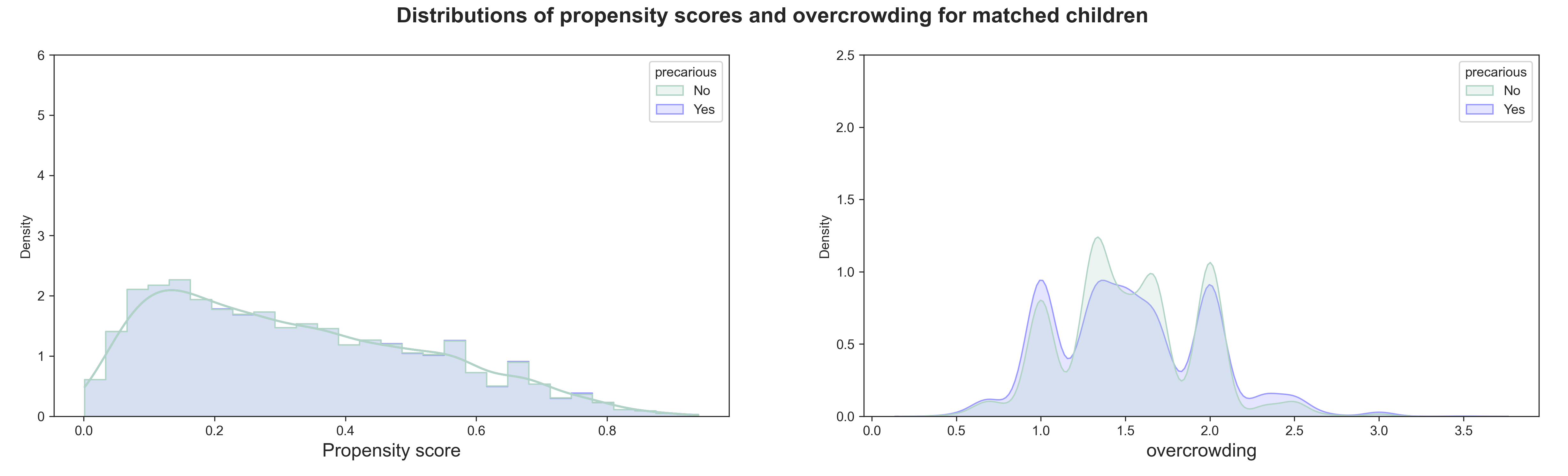
The two curves of the propensity scores now almost perfectly overlap, meaning that we perform a good matching between groups. Compared to the plots above, we can notice that the paired children are those at the intersection of both distributions. Now, the distribution of overcrowding is almost identical between both groups as well, which means that the two subpopulations are very similar except for the treatment!

Average treatment effect

Now that matching is done, we can quantify the effect of the treatment on education, health and happiness. To do so, we average the difference of each matched pair of children for different indicators of these three outcomes. ATE is given as a number between -1 and 1:

• -1: the treatment has a maximum negative effect,
• 0: the treatment has no effect,
• 1: the treatment has a maximum positive effect on the given outcome.

We also compute 95% confidence intervals, which contain the ATE with a 95% chance. Thus, ATEs will be considered significant only if 0 (no effect) is not in this interval.

Effect of precarious living conditions on education, health & happiness

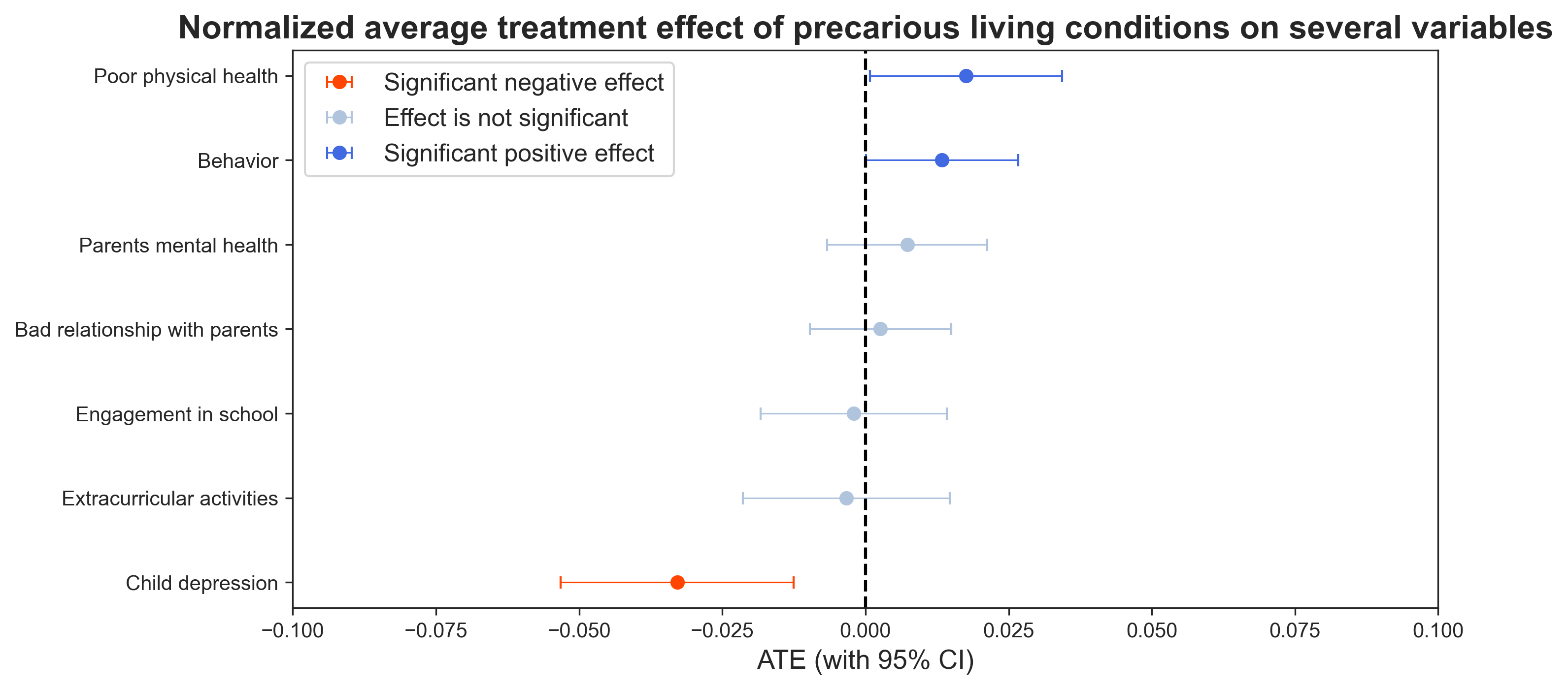
So, what is the impact of precarious conditions and which outcomes does it affect the most?

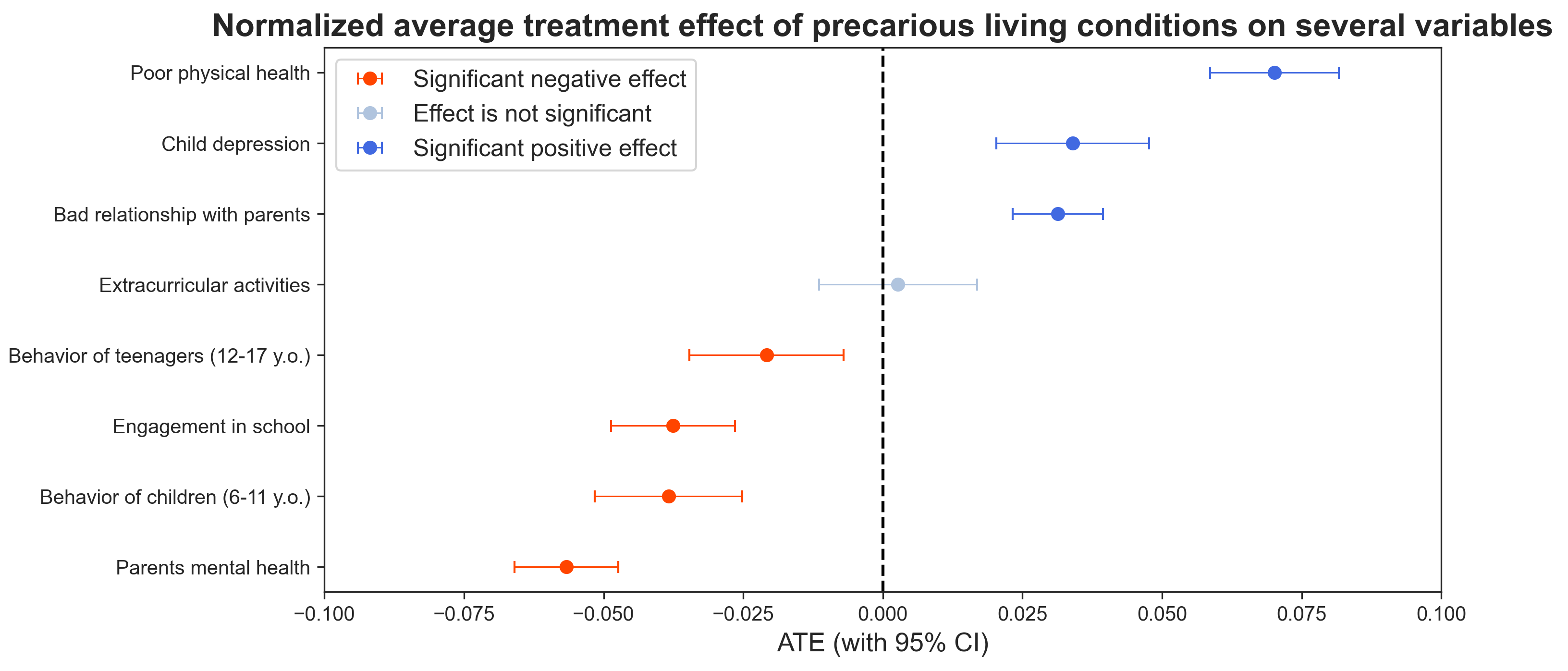
Looking at this plot, we can conclude that housing precarity strongly increases poor health and depression. It also increases bad parental relationship, even though the effect is less pronounced.

A strong negative effect appears on parents mental health, and mild negative effects are shown for school engagement and children behavior. We can notice that the behavior of younger children seems more impacted than the behavior of older ones. If you’re still interested, keep reading, we will further study differences in age groups later!

In summary, children living in precarious environments tend to have worse physical condition and mental health (so do the parents), are less involved in school and show behavioral problems and bad relationship with their parents.

Note that we included a control variable, the extracurricular activities, that we used in the propensity score computation, to make sure it was well distributed across both populations (indeed its linked ATE is not significant).

Differences across age groups

Lastly, we will check whether an age group is more affected than another by the effects we just observed. We split the population between children (aged 6 to 11) and teenagers (aged 12 to 17). We can compute the ATE of precarious conditions again on these two age groups, as well as their differences.

Let’s see what it shows:

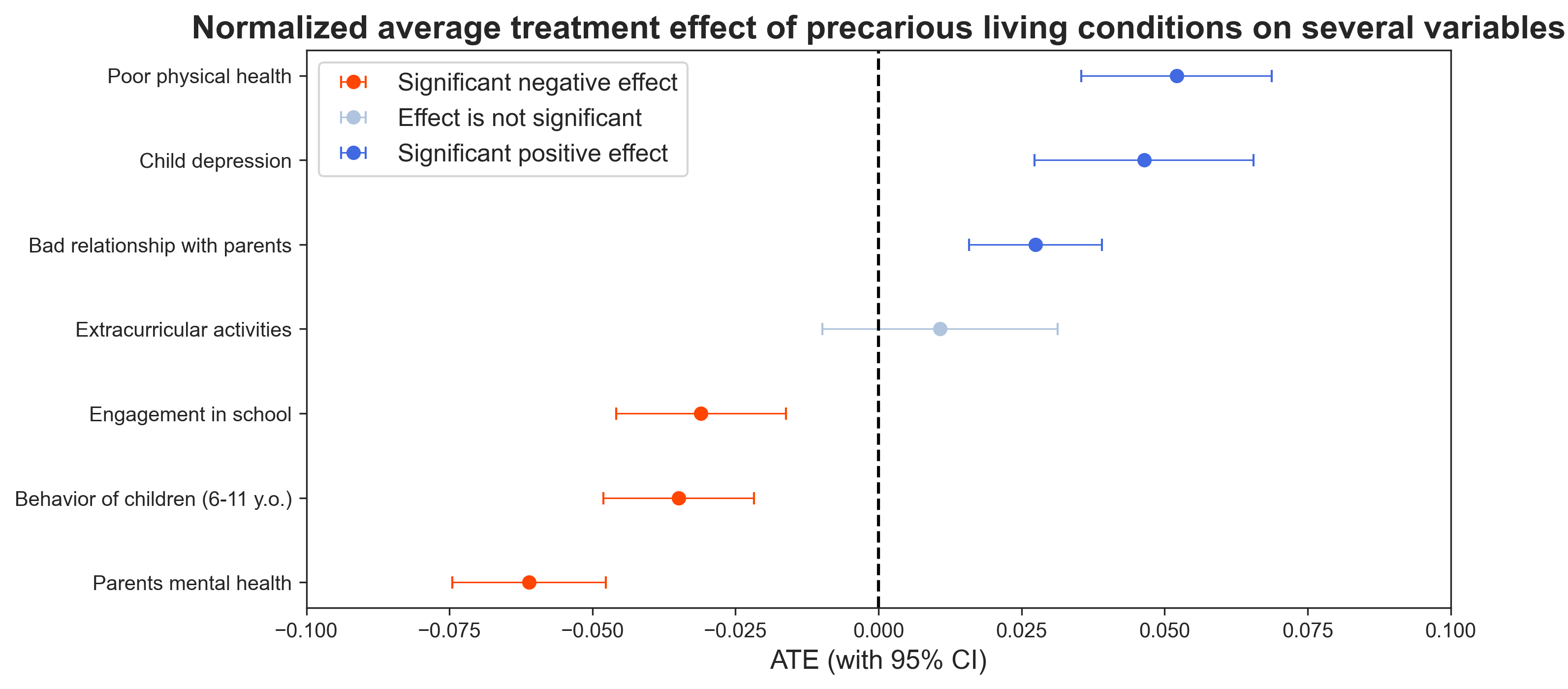
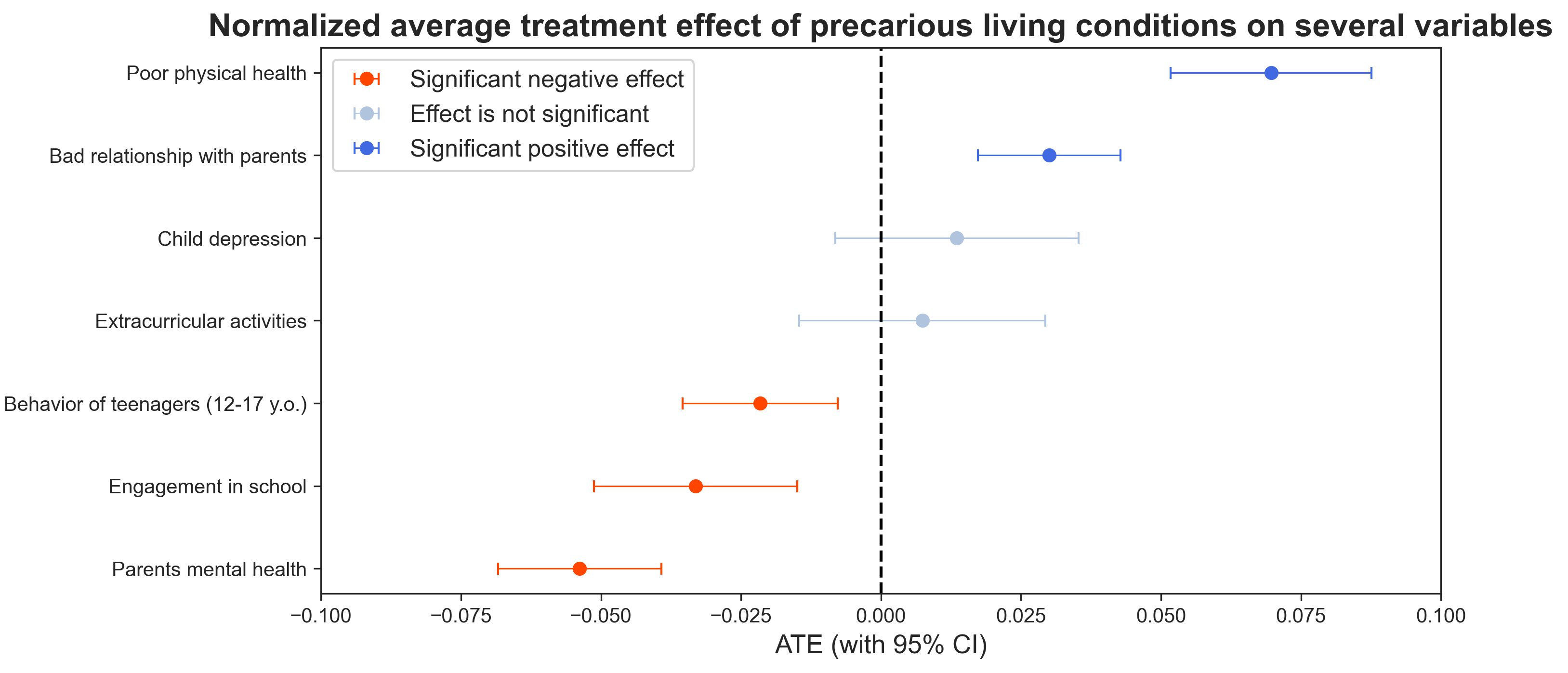
It seems that younger children’s mental health is more impacted by precarity than teenagers’. Indeed it is interesting to see that the effect on depression score is not significant for teenagers. However, recall that depression scores increase with age! We can conclude that the augmentation in depression occurence in teenagers is not particularly specific to their housing conditions.

On the other hand, the physical health of teenagers is more harshly impacted.

Regarding behavior, younger children that live in a precarious environment show more behavioral problems than teenagers.

The other variables are not significant. Thus, we can conclude that precarious living conditions affect children more than teenagers for mental health, while teenagers are more impacted on their physical condition. Education however does not seem to be affected differently across different age groups.

Conclusion

We are coming to the end of this study. What have we learned?

Living conditions and environment definitely play a role in children’s engagement in school as well as on their health, both physically and mentally. Moreover, precarious living conditions seem correlated with increasing health issues and depression. School performances are also affected.

This leads us to believe that improving the quality of life in these households would allow for better educational results and happier people, which highlights the importance of programs such as Piso Firme. Thus, it would be interesting to study sanitation programs in the United States and quantify their effect.

Finally, the exploration of this data raised some more questions, especially about the direction of causal links between different features. Further research could be done to try and find those.

This research was conducted in the context of a class project for the ADA course at EPFL.